Deep Learning-based Auto-Generation of Extensible Timeline

Abstract

Designers need to consider not only perceptual effectiveness but also visual styles when creating an infographic. This process can be difficult and time consuming for professional designers, not to mention non-expert users, leading to the demands of automated infographics design. As a first step, we focus on timeline infographics, which have been widely used for centuries. We contribute an end-to-end approach that automatically extracts an extensible and extendable timeline template from a bitmap image. Our approach adopts a deconstruction and reconstruction paradigm. At the deconstruction stage, we propose a multi-task deep neural network that simultaneously parses two kinds of information from a bitmap timeline: 1) the global information, which includes the representation, scale, layout, and orientation of the timeline, and 2) the local information, which includes the location, category, and pixels of each visual element on the timeline. At the reconstruction stage, we propose a pipeline with three techniques, i.e., Non-Maximum Merging, Redundancy Recover, and DL GrabCut, to extract an extensible template from the infographic, by utilizing the deconstruction results. To evaluate the effectiveness of our approach, we synthesize a timeline dataset (4296 images) and collect a real-world timeline dataset (393 images) from the Internet. We first report quantitative evaluation results of our approach over the two datasets. Then, we present examples of automatically extracted templates and timelines automatically generated based on these templates to qualitatively demonstrate the performance. The results confirm that our approach can effectively extract extensible templates from real-world timeline infographics.

Pipeline

missing — Figure 1. **An automated approach to extract an extensible timeline template from a bitmap image.** a) Original bitmap image; b) Content understanding including global and local information of the timeline; c) Extensible template contains editable elements and their semantic roles; d) New timeline (with mock-up colors) automatically generated with updated data.

Step b. Understand the content of an infographic by using a deep learning model.

Step c. Extract the extensible template based on the content understanding by using a post-processing pipeline.

Step d. The final output can be used to generate new timeline by binding with new data.

Labels of elements

We use two datasets to train the model and evaluate our approach. The first one (referred to as \(D_1\)) is a synthetic dataset. We extended TimelineStoryteller, a timeline authoring tool, to generate \(D_1\), covering all types of timeline. The second dataset (referred to as \(D_2\)) consists of real-world timelines, collected from Google Image, Pinterest, and FreePicker by using the search keywords timeline infographics and infographic timeline. \(D_2\) has more diverse styles, especially for marks, and it covers most common types of timeline.

To identify the categories of elements in a timeline, four of the coauthors independently reviewed all the timelines in our two datasets. Each of them iteratively summarized a set of mutually exclusive categories that can be used to depict elements in a timeline infographic. Gathering the reviews resulted in six categories:

Category	Explaination	Label type	Occurrence

For the elements that need to be reused, we labeled them with their bboxes and masks, which can be used to segment these elements from the original infographic for reusing. For those that need to be updated, we only labeled them with their bbox, since the contents of these elements need to be changed with updated data.

We also identified other guide elements (e.g., the text elements or marks in axes and legends) in our datasets. However, these elements only exist in \(D_1\). Thus, we decided to exclude them in our study.

Architecture

The above figure presents an overview of the complete architecture of our model that can parse both global and local information simultaneously. We further present the details of ResNeXt-FPN, Class Head, RPN, Box Head, and Mask Head, respectively.

1. ResNeXt-FPN

The figure above shows the configurations of the ResNeXt-FPN, which is used to extract multi-scale image features, in our model. ResNeXt ref_resnext achieves state-of-the-art performances in many computer vision tasks, we use ResNeXt to extract the features of a timeline infographic. It takes a 3-channel image (i.e., RGB) as input and uses one stem block and four groups of bottleneck block to extract features. The multipliers of bottleneck blocks are for ResNeXt-50. As for ResNeXt-101, the bottleneck block of the stage \(4\) is repeated \(23\) times rather than \(6\) times in ResNeXt-50. The four groups of bottleneck block output a feature hierarchy with a pyramidal shape that consists of feature maps with 256, 512, 1024, 2048 channels, respectively.

We then pass the feature maps into Feature Pyramid Network ref_fpn (FPN). FPN is a top-down architecture and can build semantically strong feature maps at multiple scales using the feature maps from ResNeXt. FPN makes our model scale-invariant and able to handle images of vastly different resolution. It outputs four feature maps with \(256d\) (i.e., 256 channels).

Please note that the input image can be any resolution (i.e., \(width \times height \)). Thus, in the figures, we only annotate the input/output with resolutions in parentheses for those requiring fixed size resolutions.

2. Class Head

We use Class Head that consists of two sibling fully connected (FC) layers to classify the type and orientation of a timeline infographic by consuming the feature maps from ResNeXt-FPN. 2D average pooling is applied for the features before they are passed to FC layers, following the well-established torchvision package. One problem here is which feature map should be used in Class Head, given ResNeXt-FPN outputs four \(256d\) feature maps. Considering that the task is to classify the entire image, we choose the last feature map that contains the strongest semantics and the largest scale. Another alternative is to use the feature map from ResNeXt (i.e., the \(2048d\) one). We used this feature map in our initial architecture to parse the global information. However, after extending our architecture to parse the local extra, we found out that using the \(256d\) features from FPN can stabilize the training and improve the performance. We regard this as an advantage of consistent gradients from the local and global information for the back propagation.

3. RPN

To parse the local information, we first feed the feature maps from the ResNeXt-FPN into a Region Proposal Network ref_fpn (RPN) to propose regions that may contain elements in a timeline image. RPN is a fully convolutional network (FCN) that simultaneously predicts element locations (by bbox) and objectness probability (i.e., whether there is an object within the bbox) in an image. It takes the four feature maps from ResNeXt-FPN as inputs and generates anchors (a set of reference bboxes) of various sizes for each feature map (e.g., \(32^2, 64^2, 128^2, 256^2\) for the \(1\)st, \(2\)ed, \(3\)rd, and \(4\)th feature map, respectively). For each grid in each feature map, RPN uses an anchor generator to generate three anchors of three aspect ratios (i.e., \(1:2, 1:1, 2:1\)). For each three anchors center at the same grid, RPN outputs a \(3d\) vector to predict their objectness probability and a \(3 \times 4d\) vector to predict their regression offsets. A region proposal creator will then process these outputs together with anchors to remove bboxes without elements and crop bboxes exceeding the boundary of the image. The remaining bboxes are then be used to extract regions of interest (RoIs) from the feature maps using a RoIAlign layer. Besides, the RoIAlign layer normalize each RoI to fixed sizes for passing it to two heads (\(7 \times 7\) for Box Head and \(14 \times 14\) for Mask Head).

4. Box Head

The Box Head follows the design in ref_fast_rcnn to use two sibling FC layers to classify the category and regress the bbox of the element within a RoI. It takes a \(256d\) feature of resolution \(7 \times 7 \) from RPN as the input and two FC layers to reduce the feature to \(1024d\). It then uses two sibling FC layers to output: 1) a \(7d\) vector that can be used to compute the category over 6 element categories and 1 "catch all" background, and 2) a \(6 \times 4d\) vector that represents 6 bbox regressions, each of which is a four-value tuple \(t = (t_x, t_y, t_w, t_h)\) for a category. We use the parameterization for \(t\) given in ref_fast_rcnn, in which \(t\) specifies a scale-invariant translation and log-space height/width shift relative to an RoI.

5. Mask Head

The Mask Head follows the design in ref_mask_rcnn to use an FCN for predicting the pixels of the element within a RoI. Specifically, it takes a \(256d\) feature of resolution \(14 \times 14 \) from RPN as the input and uses 4 Conv2D layers of \(3 \times 3\) kernels, 1 transposed Conv2D layer, and 1 Conv2D of \(1 \times 1\) kernel to output 6 binary masks of resolution \(28 \times 28\), one for each of the 6 categories. The binary masks indicate whether a pixel inside the RoI belongs to the element or not.

Training

1. Loss Functions

Our model is optimized for a multi-task loss function that consists of seven losses: \begin{equation} \begin{split} \mathcal{L} &= \lambda_1 \mathcal{L}_{{Image}_{type}} + \lambda_2 \mathcal{L}_{{Image}_{orientation}} \\ & + \lambda_3 \mathcal{L}_{{RoI}_{objectness}} + \lambda_4 \mathcal{L}_{{RoI}_{bbox}} \\ & + \lambda_5 \mathcal{L}_{{DT}_{type}} + \lambda_6 \mathcal{L}_{{DT}_{bbox}} + \lambda_7 \mathcal{L}_{{DT}_{mask}} \end{split} \end{equation}

	Target	Type	Loss	Weight

The summary of these losses is presented in the above table. The hyper-parameters \(\lambda\) control the balance between these seven task losses. We note that the losses defined on the entire image (i.e., \(\mathcal{L}_{{Image}_{type}}\) and \(\mathcal{L}_{{Image}_{orientation}}\)) are not on the same scale with other losses (which are defined on the local regions of the image). Therefore, we empirically set a smaller \(\lambda\) to them (i.e., 0.15) and follow previous works ref_fast_rcnnref_rpnref_mask_rcnn to keep other losses as 1. The detail computation of each loss is described as follows:

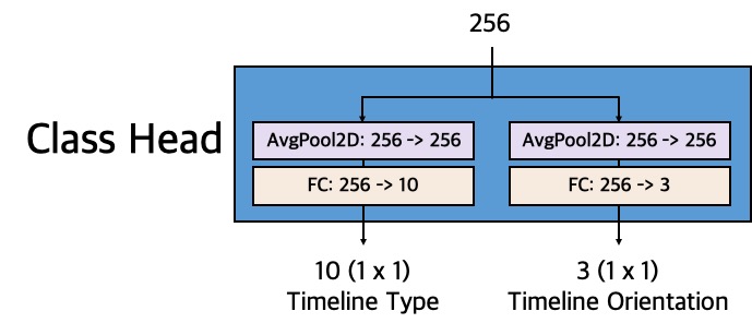
\(\mathcal{L}_{{Image}_{type}}\)

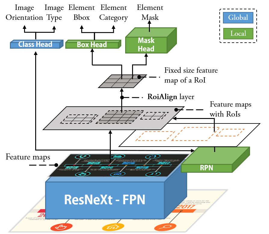
The \(\mathcal{L}_{{Image}_{type}}\), defined on the entire image, is computed using the output on the timeline type from Class Head. The output is a discrete probability distribution \(p = (p_1, ..., p_{10})\) over 10 timeline types computed by a softmax function. The timeline type classification loss is a log loss for the true type \(u: \mathcal{L}_{{Image}_{type}}(p, u) = -\log{p}_{u}\).

\(\mathcal{L}_{{Image}_{orientation}}\)

The \(\mathcal{L}_{{Image}_{orientation}}\), defined on the entire image, is computed using the output on the timeline orientation from Class Head. The output is a discrete probability distribution \(p = (p_1, p_2, p_3)\) over 3 timeline orientations computed by a softmax function. The timeline orientation classification loss is a log loss for the true orientation \(u: \mathcal{L}_{{Image}_{orientation}}(p, u) = -\log{p}_{u}\).

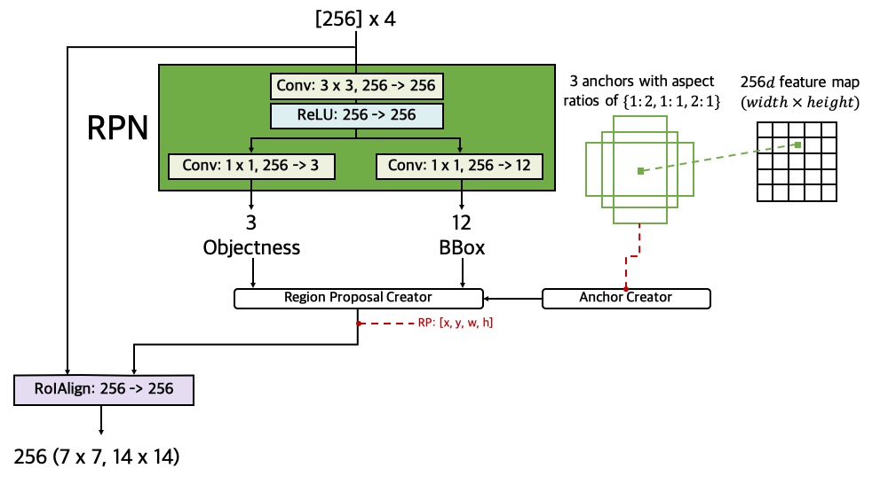
\(\mathcal{L}_{{RoI}_{objectness}}\)

The \(\mathcal{L}_{{RoI}_{objectness}}\), defined on each RoI, is computed using the output on the objectness from RPN. For each RoI, RPN uses a softmax function to compute a probability \(p\) to predict whether the RoI contains objects or not (i.e., foreground vs. background). The ground truth \(p^*\) is 1 if a RoI is foreground, and is 0 if it is background. The objectness classification loss is a log loss over two classes: \(\mathcal{L}_{{RoI}_{objectness}}(p, p^*) = - p^* \log p - (1 - p^*) \log (1 - p)\). We refer the reader to ref_rpn for more details.

\(\mathcal{L}_{{RoI}_{bbox}}\)

The \(\mathcal{L}_{{RoI}_{bbox}}\), defined on each RoI, is computed using the output on the bbox from RPN. For each RoI, RPN outputs bbox correction \(t = (t_x, t_y, t_w, t_h)\) of the anchor associated with the RoI. The regression loss is computed using Smooth \(L_1\) on the prediction \(t\) and ground truth \(t^* \): \begin{equation} \mathcal{L}_{{RoI}_{bbox}}(t, t^*) = p^* L_1^\text{smooth}(t - t^*), \end{equation} where \( L_1^\text{smooth}(x) = \begin{cases}0.5 x^2 & \text{if} \vert x \vert < 1 \\ \vert x \vert - 0.5 & \text{otherwise} \end{cases}\), and the term \(p^*\) indicates that the loss is activated only for foreground RoI (\(p^*=1\)) and is disabled otherwise (\(p^*=0\)). We refer the reader to ref_rpn for more details.

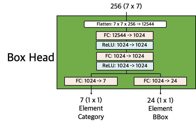
\(\mathcal{L}_{{DT}_{type}}\)

The \(\mathcal{L}_{{DT}_{type}}\), defined on each detection (i.e., DT), is computed using the output on the element category from Box Head. For each DT, Box Head uses a softmax function to compute a discrete probability distribution \(p = (p_0, p_1, ..., p_6)\) over six pre-defined element categories and a "catch all" background. The element category classification loss is a log loss for the true category \(u: \mathcal{L}_{{DT}_{type}}(p, u) = -\log{p}_{u}\).

\(\mathcal{L}_{{DT}_{bbox}}\)

The \(\mathcal{L}_{{DT}_{bbox}}\), defined on each DT, is computed using the output on the element bbox from Box Head. For each DT, Box Head outputs 6 bbox regression corrections, \(t^k = (t^k_x, t^k_y, t^k_w, t^k_h)\) indexed by \(k\), one for each of the 6 categories. We use the parameterization for \(t^k\) given in ref_fast_rcnn, in which \(t^k\) specifies a scale-invariant translation and log-space height/width shift relative to a region proposal (RoI). Similar to \(\mathcal{L}_{{RoI}_{bbox}}\), the regression loss \(\mathcal{L}_{{DT}_{bbox}}\) is also computed using Smooth \(L_1\): \(\mathcal{L}_{{RoI}_{bbox}}(t^u, t^*) = [u > 0] L_1^\text{smooth}(t^u - t^*) \), where \(t^u\) is the predicted bbox correction of the true category \(u\) and \(t^*\) is the ground truth. The Iverson bracket indicator function \([u > 0]\) evaluates to 1 when \(u > 0\) and 0 otherwise, which means the loss is only activated on the foreground predictions (\(p_1\) to \(p_6\)), since the "catch all" background class is labeled \(u = 0\) by convention. We refer the reader to ref_fast_rcnn for more details.

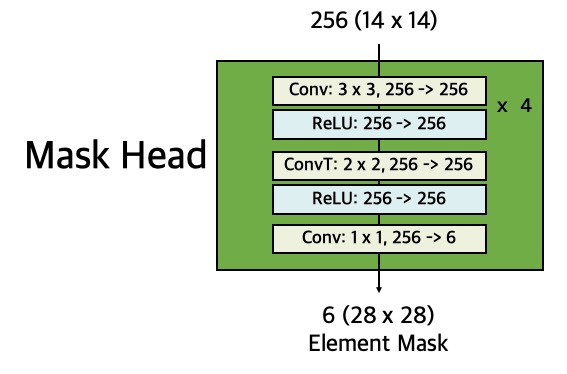
\(\mathcal{L}_{{DT}_{mask}}\)

The \(\mathcal{L}_{{DT}_{mask}}\), defined on each DT, is computed using the output of Mask Head. For each DT, Mask Head outputs 6 binary masks of resolution \(m \times m \) (defined as a hyper parameter), one for each of the 6 categories. \(\mathcal{L}_{{DT}_{mask}}\) is defined as the average binary cross-entropy loss over all pixels of a mask. Besides, for an DT associated with its ground true category \(u\), the loss is only defined in the \(u\)-th mask (other mask outputs do not contribute to the loss): \( \mathcal{L}_{{DT}_{mask}} = - [u > 0] \frac{1}{m^2} \sum_{1 \leq i, j \leq m} \big[ p^*_{ij} \log p^u_{ij} + (1-p^*_{ij}) \log (1- p^u_{ij}) \big] \), where \(p^*_{ij}\) is the label of a pixel \((i, j)\) in the true mask and \(p^u_{ij}\) is the predicted label of the same pixel for the true category \(u\); the term \([u > 0]\) works in the same manner as in \(\mathcal{L}_{{DT}_{bbox}}\). We refer the reader to ref_mask_rcnn for more details.

2. Hyper parameters

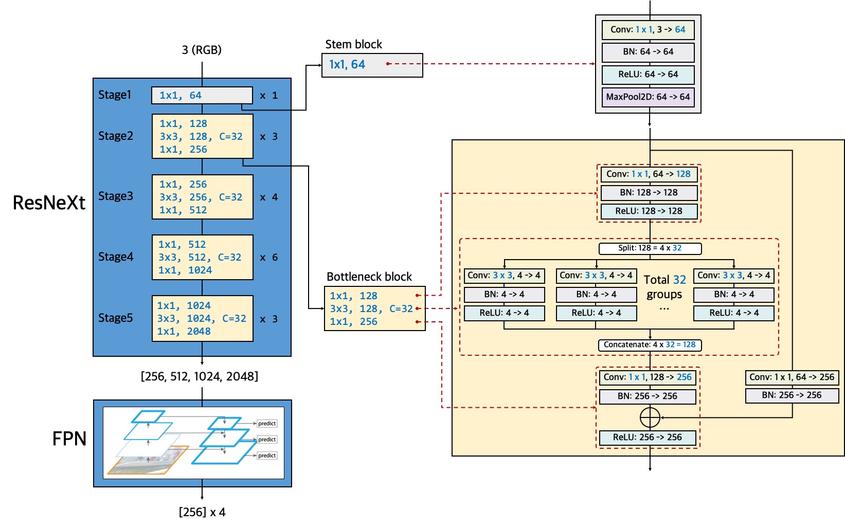
We implemented two types of CNN backbone for our model, namely, ResNeXt-101 and ResNeXt-50. Below are the hyper parameters we used to train our models with ResNeXt-101 and ResNeXt-50, respectively.

        MODEL:
            META_ARCHITECTURE: "GeneralizedRCNN"
            WEIGHT: "catalog://ImageNetPretrained/FAIR/20171220/X-101-32x8d"
            BACKBONE:
                CONV_BODY: "R-101-FPN"
                OUT_CHANNELS: 256
            CLASSIFIER:
                NUM_CLASSES: 10 
            CLASSIFIER2:
                NUM_CLASSES: 3
            RPN:
                USE_FPN: True
                ANCHOR_STRIDE: (4, 8, 16, 32, 64)
                PRE_NMS_TOP_N_TRAIN: 2000
                PRE_NMS_TOP_N_TEST: 1000
                POST_NMS_TOP_N_TEST: 1000
                FPN_POST_NMS_TOP_N_TEST: 1000
            ROI_HEADS:
                USE_FPN: True
                BATCH_SIZE_PER_IMAGE: 256
            ROI_BOX_HEAD:
                POOLER_RESOLUTION: 7
                POOLER_SCALES: (0.25, 0.125, 0.0625, 0.03125)
                POOLER_SAMPLING_RATIO: 2
                FEATURE_EXTRACTOR: "FPN2MLPFeatureExtractor"
                PREDICTOR: "FPNPredictor"
                NUM_CLASSES: 7
            ROI_MASK_HEAD:
                POOLER_SCALES: (0.25, 0.125, 0.0625, 0.03125)
                FEATURE_EXTRACTOR: "MaskRCNNFPNFeatureExtractor"
                PREDICTOR: "MaskRCNNC4Predictor"
                POOLER_RESOLUTION: 14
                POOLER_SAMPLING_RATIO: 2
                EXCLUDE_LABELS: (0, 3)
                RESOLUTION: 28
                SHARE_BOX_FEATURE_EXTRACTOR: False
            RESNETS:
                STRIDE_IN_1X1: False
                NUM_GROUPS: 32
                WIDTH_PER_GROUP: 8
            MASK_ON: True
            CLASSIFIER_ON: True 
            CLASSIFIER2_ON: True
        INPUT:
            MIN_SIZE_TRAIN: 833
            MAX_SIZE_TRAIN: 1024
            MIN_SIZE_TEST: 833 
            MAX_SIZE_TEST: 1024
        DATALOADER:
            SIZE_DIVISIBILITY: 32
            ASPECT_RATIO_GROUPING: False
        SOLVER:
            BASE_LR: 0.005
            WEIGHT_DECAY: 0.0001
            STEPS: (56000, 76000)
            # Epoch = (MAX_ITER * IMS_PER_BATCH) / #dataset
            MAX_ITER: 84000
            IMS_PER_BATCH: 4
            CHECKPOINT_PERIOD: 10000
        MODEL:
            META_ARCHITECTURE: "GeneralizedRCNN"
            WEIGHT: "catalog://ImageNetPretrained/MSRA/R-50"
            BACKBONE:
                CONV_BODY: "R-50-FPN"
                OUT_CHANNELS: 256
            CLASSIFIER:
                NUM_CLASSES: 10 
            CLASSIFIER2:
                NUM_CLASSES: 3
            RPN:
                USE_FPN: True
                ANCHOR_STRIDE: (4, 8, 16, 32, 64)
                PRE_NMS_TOP_N_TRAIN: 2000
                PRE_NMS_TOP_N_TEST: 1000
                POST_NMS_TOP_N_TEST: 1000
                FPN_POST_NMS_TOP_N_TEST: 1000
            ROI_HEADS:
                USE_FPN: True
                BATCH_SIZE_PER_IMAGE: 256
            ROI_BOX_HEAD:
                POOLER_RESOLUTION: 7
                POOLER_SCALES: (0.25, 0.125, 0.0625, 0.03125)
                POOLER_SAMPLING_RATIO: 2
                FEATURE_EXTRACTOR: "FPN2MLPFeatureExtractor"
                PREDICTOR: "FPNPredictor"
                NUM_CLASSES: 7
            ROI_MASK_HEAD:
                POOLER_SCALES: (0.25, 0.125, 0.0625, 0.03125)
                FEATURE_EXTRACTOR: "MaskRCNNFPNFeatureExtractor"
                PREDICTOR: "MaskRCNNC4Predictor"
                POOLER_RESOLUTION: 14
                POOLER_SAMPLING_RATIO: 2
                RESOLUTION: 28
                SHARE_BOX_FEATURE_EXTRACTOR: False
            MASK_ON: True
            CLASSIFIER_ON: True 
            CLASSIFIER2_ON: True 
        INPUT:
            MIN_SIZE_TRAIN: 833
            MAX_SIZE_TRAIN: 1024
            MIN_SIZE_TEST: 833
            MAX_SIZE_TEST: 1024
        DATALOADER:
            SIZE_DIVISIBILITY: 32
            ASPECT_RATIO_GROUPING: False
        SOLVER:
            BASE_LR: 0.005
            WEIGHT_DECAY: 0.0001
            STEPS: (56000, 76000)
            # Epoch = (MAX_ITER * IMS_PER_BATCH) / #dataset
            MAX_ITER: 84000
            IMS_PER_BATCH: 4 
            CHECKPOINT_PERIOD: 10000

Examples

1. Examples outputted from the model and refined by DL GrabCut.

After applying Non-Maximum Merging and Redundancy Recover, we visualize the final predicted category, bbox, and mask of each element on timelines. We then apply DL GrabCut and convert the timeline infographics to greyscale images for a clear demonstration. Please note that the aliasing of some borders of masks is caused by the rendering method we used (i.e., the findCountor in openCV.)

2. Supplemental examples

In this section, we provide additional examples from ablation studies to indicate some properties of the model.

Examples of parsing infographics with natural and graphical elements

In an infographic, a common practice is to show objects with photos and annotate them with graphical shapes. Such kind of hybrid components requires a model that considers the characteristics of natural and graphical elements. Although our datasets do not include natural elements, we are interested in the performance of our model on timelines contain graphical and natural elements. Thus, we randomly substitute some graphical marks with photos of animals and then feed them to our model.

In the Fig.a above, we substitute all annotation icons with animal photos and randomly add additional animal photos for disruption. The results show that our model can still correctly classify these animals as annotation icons. We regard this performance as a benefit of the ImageNet pre-trained network.

In the Fig.b, we further substitute all event marks with animal photos to see whether the model can classify them as event marks. Interestingly, our model can finish the task perfectly: although the cats look identical, our model classifies the cats that randomly distributed in the image as annotation marks, while the cats on the main body as event marks.

However, this result does not mean that the model can recognize elements based on their locations and relationships with other elements. Figure.c presents a more general case. For this infographic, which has a similar representation with a linear timeline, our model can correctly identify the annotation marks, annotation text, and annotation icons, but classifies all corncobs in the middle as annotation icons instead of event marks or main body. This example demonstrates that the DL model mainly recognizes elements based on their visual appearance, rather than their locations and relationships to other elements. Thus, for the cats on the main body in Fig.b, we conjecture that is the appearances of them together with other elements (e.g., the main body and annotation marks) around that help our model to achieve correct classifications.

These examples relate to issues about networks on images with natural and graphical elements. Besides, these examples also involve translation invariance vs. translation variance in networks. Future research is needed to understand these cases further. We discuss these issues and potential solutions in Section 7.1 in our paper.

Examples of using tricks to improve the detection results

Given our work is not aimed at high metric values, we did not optimize our model with bells and whistles, such as comprehensive data augmentation, multi-scale train/test, more advanced loss functions, and other techniques. Outside the scope of this work, we expect that such improvement skills are applicable to our model. Here we present examples to demonstrate how our model can be improved with such kind of techniques.

The Fig.d shows a timeline infographic and Fig.e presents the detection results of our model. As shown in Fig.e, the annotation marks are not covered by the bboxes. Our investigation reveals that this is because the sizes of the annotation marks are too large with respect to the image size. There is no such kind of unusual large annotation marks in the training set. Thus, the model tends to use a relatively small bbox to cover the annotation marks. In Fig.f, we apply a multi-scale testing technique by extending the image (resizing also works) to reduce the relative size of the annotation marks. The model then can detect the marks correctly. Multi-scale training, which is a data augmentation strategy. is another method to tackle this kind of cases. Simply put, we can resize the training images to cover diverse sizes of annotation marks.

Figure.h is a greyscale timeline and Fig.i shows the detection results. As shown in the enlarging views in the top of Fig.i, some event marks, whose colors are similar to the background color, are undetected or incorrectly detected as a part of the annotation text. We discover that the lacking of greyscale training data is the major reason, because in timelines with RGB channels it is unusual to have event marks with colors similar to the background color. Thus, we randomly add some colors to the undetected event marks (Fig.j). The model successfully detects these marks as our expected (Fig.k). To handle this kind of cases, a data augmentation strategy that converts RGB images to greyscale images can be applied in training samples.

Both these two representative cases (i.e., the large size and greyscale examples) can be addressed by data augmentation techniques. Besides the data aspect, there are other enhancement techniques for networks, such as OHEMref_OHEM, focal lossref_focal_loss, soft-NMSref_soft_nms, etc. We leave this improvement techniques for future work.

Reference

Saining Xie, Ross Girshick, Piotr Dollár, Zhuowen Tu, Kaiming He. "Aggregated Residual Transformations for Deep Neural Networks." In Proc. IEEE CVPR. 2017.

Tsung-Yi Lin, Piotr Dollár, Ross Girshick, Kaiming He, Bharath Hariharan, Serge Belongie. "Feature Pyramid Networks for Object Detection." In Proc. IEEE CVPR. 2017.

Ross Girshick. “Fast R-CNN.” In Proc. IEEE ICCV. 2015.

Shaoqing Ren, Kaiming He, Ross Girshick, and Jian Sun. “Faster R-CNN: Towards Real-time Object Detection with Region Proposal Networks.” In Proc. NIPS. 2015.

Kaiming He, Georgia Gkioxari, Piotr Dollár, and Ross Girshick. "Mask R-CNN." In Proc. IEEE ICCV. 2017.

Abhinav Shrivastava, Abhinav Gupta, Ross Girshick. "Training Region-based Object Detectors with Online Hard Example Mining." In Proc. IEEE CVPR. 2016.

Tsung-Yi Lin, Priya Goyal, Ross Girshick, Kaiming He, Piotr Dollár. "Focal Loss for Dense Object Detection." In Proc. IEEE ICCV. 2017.

Navaneeth Bodla, Bharat Singh, Rama Chellappa, Larry S. Davis. "Soft-NMS -- Improving Object Detection With One Line of Code." In Proc. IEEE ICCV. 2017.

Towards Automated Infographic Design: Deep Learning-based Auto-Extraction of Extensible Timeline